Upside Down CAPM, Part 2: The value of growth
In part 1, I suggested an empirical starting point for the Capital Asset Pricing Model - that expected returns on at-risk capital are stable. In other words, changes in equity prices aren’t generally the result of changing discount rates. They result from changes in real economic conditions and expectations.
Interest rates reflect the discount that savers must accept to receive guaranteed cash flows on fixed income securities. Fixed income savers are deferred consumers. Risk free interest rates are not a very useful guide for estimating fair value of other assets.
There are two simple equations here. First, the CAPM equation:
ERi = Rf + ERP
This is just a simple accounting identity for risk. Total expected returns on at-risk assets (ERi) are a combination of risk free yields (Rf, which can be measured in the marketplace) and the equity risk premium (ERP, which cannot)
Second, the total expected returns on at-risk assets are a combination of current earnings plus the expected growth rate of future earnings:
ERi = (Earnings / Price) + g
I’m not sure if these are strong enough assertions to be axioms, but let’s call them rules of thumb.
Real ERi is a relatively constant 6% over time, which means that Rf and ERP are negatively correlated.
Rf is positively correlated with expected growth.
Because of points #1 and #2, the earnings yield is positively correlated with the equity risk premium.
Really, this is mostly a subtle issue of causality. Everyone agrees that when investors are risk seeking, price/earnings ratios rise and earnings/price yields decline.
If we substitute the CAPM components for ERi:
Rf + ERP = (Earnings / Price) + g
and solve for price:
Price = Earnings / (Rf - g + ERP)
The conventional approach is to say that prices are driven up and down by stimulus and austerity, greed and fear. Prices can go up if stimulus pushes down Rf or if greed pushes up g. That presumes a world where Rf and g are negatively correlated, where, for instance, cheap money fuels higher growth expectations. Empirically, that is not the world we live in. g is positively correlated with Rf and negatively correlated with ERP.
In either model, when g goes up, prices go up. But, in the upside-down CAPM, the interaction with interest rates is reversed from the conventional approach. The conventional model lends itself to a corrosive presumption that irrational waves of herding behavior or federal manipulation are what pushes prices up and down. The upside down model fits into the traditional paradox of growth economics - the paradox that North, Wallis, and Weingast describe in Violence and Social Orders.
We know how high-trust societies work and how they engender shared prosperity. We can describe them. But we don’t know how to create them.
That is true in the bigger picture. South Korea and Taiwan happened. We could see how the transition works. But, we haven’t figured out how to plunk down a game plan in Moscow and do a game reset where contracts are honored and long term investments in human and physical capital are taken on in confidence that they will be valued and honored.
Cyclical or generational fluctuations in economic growth represent the same problem at a narrower scale. If the economy isn’t growing, corporations aren’t going to fund their innovative R&D programs. But if corporations don’t fund their R&D, the economy won’t grow.
The centrally managed money supply is intended to strong arm those sentiments into a high trust / shared growth regime. But, communicating monetary policy through interest rates is incoherent. Somehow, we have managed some success at taming the business cycle while using that incoherent framework.
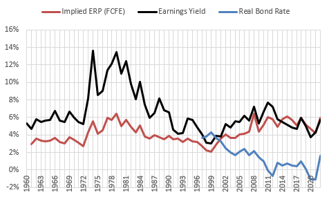
My 3 rules of thumb are reflected in Figure 1. Here, I show the real bond yield for as long as we have had a market for real yields. At the peak of the 1990s tech boom, real Treasury yields were higher than the earnings yield on the S&P 500. That is because growth expectations were very high and so ERP was very low.
The conventional approach will point to those high growth expectations as signs of irrational exuberance. There was a lot of exuberance, and certainly some of it was irrational. But, what the conventional approach leaves underappreciated is that fixed income yields were very high. Demand for deferred consumption was low. Supply of at-risk capital was high. Even though the boom ended and growth expectations later fell, we are still all basking in the flood of innovations that came from those investments.
Since then, fixed income yields, growth expectations, and growth have all declined. And, because of the 3 rules of thumb, ERP and the earnings yield have both risen from their late 1990s lows.
We don’t have market prices for real bond yields before the late 1990s, but Aswath Damodaran does estimate earnings yields and ERP back to 1960. Their general movements were also positively correlated then. (I think the main reason that the earnings yield was especially elevated in the inflationary 1970s was because in an inflationary environment, future taxation on inflationary capital gains requires a higher yield to provide the same future after-tax returns.)
ERP and the earnings yield both increased during the 1970s when real growth faltered. Sentiment about growth was negative in the 1970s, but it is a little tricky to see the lower growth in the data. In the recent period, lower growth has been associated with slower expansions. In the 1970s, lower growth was associated with more frequent recessions.
Figure 3 compares total real returns on the S&P 500 and real growth in GDP per worker, over rolling 10 year periods.
Growth expectations, risk aversion, and experienced growth are all interconnected in this mysterious collective action problem. When savers are confident about growth and invest in growth, both savers and workers benefit. And, even deferred consumers benefit. Because, remember, when growth expectations are high, the equity risk premium is low, which means that fixed income yields are high. It’s a win-win-win. And, the upside-down CAPM helps to see it all working together.
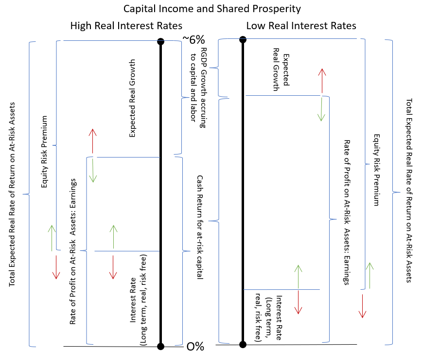
Figure 3 lays out how all of the versions of income and growth are related within that stable 6% real return of at-risk capital.
On the right side is the low-rate context. Risk free savers (deferred consumers) earn little. Wages grow slowly. And, cash returns to capital are high.
On the left side is the high-rate context. Risk free savers earn more. Wages grow quickly. And cash returns to capital are low, because more of their returns come from growth. The returns from growth are shared by all - capital, labor, and consumer.
The upside-down CAPM helps to see all of this working together - sentiment and action determining the returns to both equity and fixed income and influencing real growth.
Seeing it this way highlights the value of the growth of at-risk capital. In the aggregate, all of the benefits of increased at-risk capital are externalities. The stability of expected total returns over time is the empirical clue to that conclusion.


What falsifiable predictions does your model make?