"Reassessing the role of supply and demand on housing bubble prices"(Part 1)
New paper!
The third paper in my series on the relationships between incomes, rents, and home prices is posted.
First, I am getting great feedback on the previous paper. It really does help to understand the forces that push home prices up to unsustainable levels. I encourage you to read it and share! You will be glad that you did!
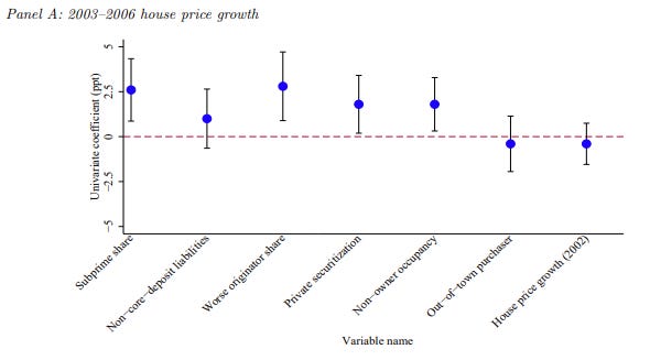
In that paper, I developed a proxy variable for metropolitan area supply constraints at any point in time, and in this paper, I use that variable to review the evidence about the causes of changing home prices from 2002 to 2010. I reference “What Drove the 2003-2006 House Price Boom and Subsequent Collapse? Disentangling Competing Explanations” by Griffin, Kruger, and Maturana for the framework I use. Figure 1 is from their paper.
They compare 7 variables (4 “credit supply” variables and 3 “speculation” variables). The figure shows the correlation of one standard deviation in each factor with home prices from 2003 to 2006. So, for instance, in ZIP codes where subprime lender market share was one standard deviation above average, home prices tended to rise by an additional 2.6%.
They find that, after adding various controls, including income and metropolitan area fixed effects, the credit supply variables have the strongest correlations with rising prices. But, the controls are doing a ton of work here. The r-squared estimates on these 7 regressions (how well the estimates using these variables fit with the measured price changes, on a scale of 0 to 1) range from .844 to .847. The fit is practically unaffected by the use of these variables. Much of the fit comes from the metro fixed effects (the differences between metro areas). In their data set, the average price change was 46.3% and the standard deviation was 30.3%. The standard deviation of price changes between metros (excluded from the analysis with metro area fixed effects) was 31.4% and within metros it was 13.3%.
So, even before I approach this with my new variable, I think it is notable how much of the story of the housing boom has been systematically ignored by the academy. This debate between the credit supply school (represented by their first 4 variables - “Loose lending pushed prices up.”) and the passive credit or speculation school (represented by their last 3 variables - “Speculation pushed up prices, and that sometimes used credit.”) is about a vanishingly small part of the story. Maybe that is necessary, in order to carefully estimate the power of these variables. But, even if it is necessary, ignoring the difference between Dallas and Los Angeles in a debate about the factors moving home prices from 2002 to 2006 is an extreme form of “feeling parts of the elephant”. The debate about what exactly the elephant is has been overwhelmingly driven by an argument over the length of its tail.
Even the results they report here are small. The two strongest findings - subprime share and worse originator share (lenders with poor underwriting) - claim to be associated with a bit less than a 3% change in home prices. In a fit of pique, on a data set with average price changes of 46% and a standard deviation of 30%, one might be forgiven for exclaiming “Who cares?!” The rejoinder to that is some version of, “If this factor explains so much of the tail, imagine how much it might explain of the rest of the creature!”
Another rhetorical form taken with these sorts of findings is to treat local supply conditions as a fixed factor that the other factors act on. So, where supply conditions interact with credit variables, the conclusion is “Credit access was associated with a boom and bust, and it was especially so where supply conditions were constrained.” That conclusion is purely a rhetorical choice, not an empirical one. We could just as easily report that constrained supply can lead to price volatility, and when credit is loose, supply constraints increase prices even more.
One big problem is that, as far as I know, nobody has a variable for the effect of supply conditions that changes in real time. THIS IS THE PROBLEM MY PREVIOUS PAPER SOLVES. And, if I may be so bold, I think this can be very useful! Without my variable, even if they wanted to rhetorically center supply constraints, what variable could they point to which could do that independently of an interaction with these demand variables? I have found that variable!
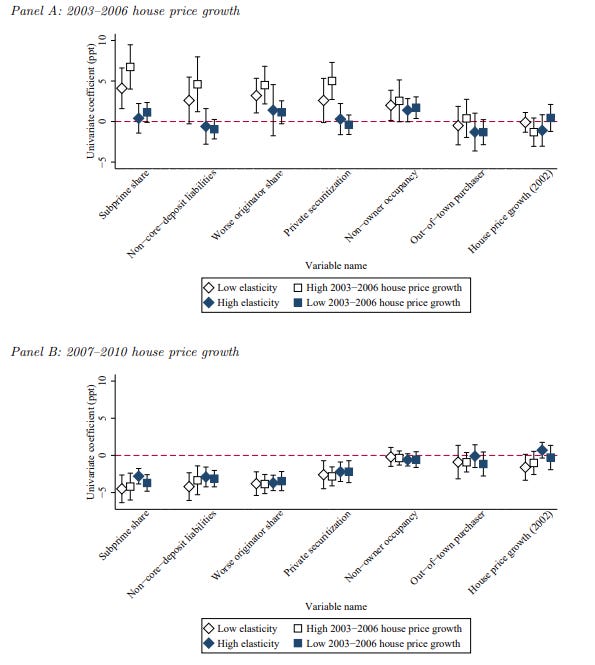
Figure 2 here is the figure where Griffin, Kruger, and Maturana do that analysis.
There are figures here for the boom period and the bust period, and GKM use these figures to argue 2 points. The first is the point above (the credit variables were especially strong factors moving prices where supply was constrained). The second is that the credit variables were associated with declining prices in both types of cities. They note that the credit variables were associated with higher home purchase volumes during the boom, and so they consider this additional evidence of the power of the credit variables. Where supply was constrained, aggressive lending led to rising prices. Where supply wasn’t constrained, it led to more construction. In either case, when the credit bubble ended, prices declined as a result.
One problem with this analysis is their variable for production. They use data for purchases of existing homes. Data on new construction wouldn’t be applicable at the ZIP code level, so this is understandable. But, I just don’t think it is convincing. Why would home prices decline in a market where prices never increased substantially, but homes had traded hands more often? A better variable to use here is new housing production, but it is hard to estimate supply relative to demand, and that variable can’t really be applied at a scale smaller than the metro area.
I have written a bit on this. There just isn’t much evidence that construction rates were higher in moderately priced cities than they were in the volatile markets. And, in fact, by 2007, when their “bust” period begins, in places where prices had been moderate and where construction had never really increased, construction was already in deep decline. There is no evidence of a glut of supply, and GKM follow the universal convention on the matter by failing to interrogate that question.
Readers of this newsletter will know what alternative explanation I have for the universal decline in home prices associated with constrained credit. There was a novel change in mortgage underwriting, reaching well into prime borrowers, that universally lowered home values in credit constrained neighborhoods in every city after 2007. It left a signature on home values distinct from the rise and fall of the subprime credit boom. I will write more on that in later posts.
So, first things first, Figure 3 shows the effect of 2 credit supply variables and 2 speculation variables that I used. This is not a direct replication of GKM. I use the log change in price/income ratios as the dependent variable. I have a somewhat different data set. My credit variables are FHA share and the denial rate on new loans. Also, while they do a number of different regressions, the figures above are based on regressing each variable separately, and the regressions I will discuss of my data are of multi-variate regressions with all variables. And there are other small differences.
You can see that, using metro area fixed effects and income controls, my variables show correlations in the same ballpark as theirs. The pre-trend price change in my data is a stronger than theirs. My strongest credit supply variable has a similar effect scale as theirs.
In Figure 4, I add my supply conditions variable. All of these variables represent the pre-existing conditions of each ZIP code in 2002. The supply variable also represents supply conditions in 2002 (technically, the slope of the price/income line from my previous paper interacted with ZIP code income). I had expected that by attributing all the causality to credit variables, they had overestimated the scale of their importance. So, by adding my supply variable, I thought it might decrease the estimated importance of the credit variables. I was wrong! It increased their association with price changes.
By including the supply variable, one standard deviation change in FHA market share is associated with a 6% price increase instead of a 3% increase. The denial rate also becomes a positive factor. But, the demand factors are all dwarfed by the scale of the effect of supply constraints. (And, the differences between metro areas still account for more difference than any of these variables do. As I will discuss in later posts, I think by using my added supply variable, the remaining metro area differences may convey more useful information.)
So, what’s going on? I think there was a credit boom from 2002 to 2006. My variable allows the credit boom to be better identified! But, I also think that credit boom was much less important than it has been made out to be. I will argue, in fact, that it was orthogonal to the supply-constraint problem, or even mitigating it somewhat. Discussing that will require more than one post. In the meantime, you can read the paper. Or, if you haven’t read the previous paper, start there. I’m confident you will find it useful and/or interesting. And, if the previous set of posts or the papers are too long, here is a very short slide deck with some of the tl;dr’s.
More posts to follow.


