Metro Area Housing Analysis Packages: Part 1

I have created a standardized version of basic analysis for each major metropolitan area. I am making these available, temporarily, for a significantly discounted price, in order to kick start this product and to give some of you a chance to get your feet wet regarding how to use my model in your operational and investment decisions.

These reports will cover more than 100 of the largest housing markets.

Over the next few posts, I am going to walk through the data for a sample city to show how the model works and how you can use this information to gain an advantage on capital allocation and investment decisions. I previously hinted at this framework in a series of posts about home and land valuations.

In the monthly Erdmann Housing Tracker data, I use price/income ratios. It can differentiate between 3 causes of home price changes.

Price/income ratios in the richest neighborhoods in a metro area reflect cyclical price deviations. Cyclical deviations tend to affect prices across a region proportionately. Since the richest neighborhoods are not sensitive to supply or credit conditions, they provide a window into cyclical changes.

Looser lending raises price/income ratios more in poorer neighborhoods and tighter lending compresses prices more in poorer neighborhoods.

When supply conditions are inelastic, meaning not sensitive to price, markets must clear through displacement - families choosing to move to cheaper neighborhoods or out of the region altogether. Families resist that, and so they are willing to pay higher rents under those conditions. Pressure on rents under those conditions is regressive. Rents rise more in poorer neighborhoods than in richer neighborhoods and prices reflect that.

You can see the effect of these 3 factors in Phoenix, in Figure 1. The price/income ratio across the region used to be about 3x, before distortions in credit access and local supply constraints broke the market. In 2005, Phoenix experienced a tremendous cyclical boom. So the price/income ratios across the entire region rose to about 5x. That was about 2 points higher than normal across the region. That was unlikely to be sustainable, and it wasn’t sustained. By 2011, price/income ratios in the richest neighborhoods had corrected back to about 3x. But, on top of that, the mortgage crackdown pushed price/income ratios in the poorest neighborhoods down to nearly 2x.

Figure 1

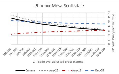
Since then, cyclical shifts have been relatively tame, so price/income ratios in Phoenix have been tethered at near 3x at the right end of Figure 1. The subsequent supply collapse raised the left end from 2x to about 6x because of regressive rent inflation.

The price/income ratio of every neighborhood in Phoenix today is mostly a product of where neighborhood income falls on that line, plus some idiosyncratic differences between neighborhoods. The idiosyncrasies used to be everything. Now they are a minority of the explanation for a given home’s value.

Estimating unsustainable land inflation

Using prices instead of price/income ratios allows for a different approach, which focuses on excess land value. Below, and in following posts, I will be referencing a single sample city.

Figure 2 shows home prices across its ZIP codes in January, for the years 2000 through 2004. This period is an example of a normal marketplace with mainly cyclical changes.

That period was cyclically ascendant. So, each year, home prices increased proportionately across the region. Here, that means that the pattern of prices across ZIP codes is tethered at the left end. Think of this as the value of a marginal lot carved out of farmland on the city’s edge, with access to utilities but no particular locational value. In this city, that tended to be between $20,000 and $30,000.

Figure 2

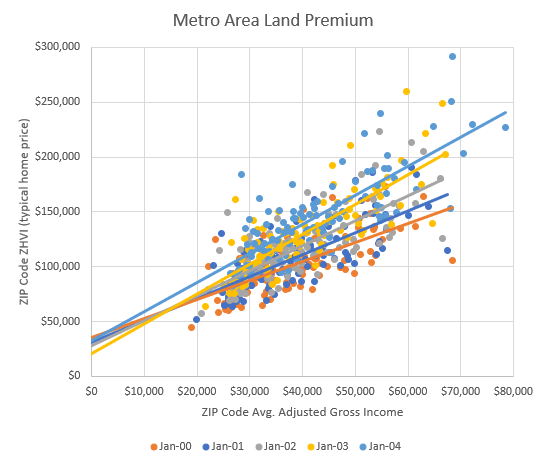
I estimate that sometime during the year 2002, this market was what I would call cyclically neutral. But, regardless of whether homes in this city were 10% above or below cyclically neutral, the basic market price of the marginal lot was stable. The price/income ratio measure moved up and down across the whole region. Prices were tethered at about $25,000 above the origin and the slope of the valuation line went up or down across incomes. There were variations in the prices families were willing to pay for the level of amenities associated with neighborhoods of various income levels.

So, in the typical ZIP code with average income of $60,000, in January 2000, the typical home cost about $25,000 plus 1.7 x 60,000. In January 2002, it was about $25,000 plus 2.3 x 60,000. In January 2004, it was about $25,000 plus 2.7 x 60,000.

That was basically all cyclical inflation. After marginal land costs, families across the city sorted into the stock of homes, with its various choices in neighborhood amenities, size and quality of units, and location, in a way that cost 1.7x the typical family’s income in 2000 and 2.7x the typical families income in 2004. Quite a large cyclical shift. Though, keep in mind, that price ratio in 2000 was very low. Most of the shift was from an underpriced market back toward normal price ratios.

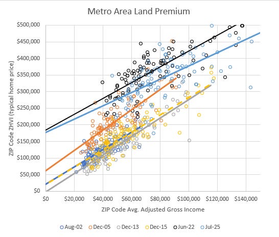
In Figure 3, I reference August 2002 as a cyclically neutral normal market for this city. By December 2005, cyclical froth had increased the price/income coefficient to 3.1x. But, also lots across the city had increased in value, to more than $60,000. In 2005, much of the inflation was probably related to the credit boom. It acted especially strongly in this city, leading to more demand for purchasing homes in poorer, credit constrained neighborhoods, inflating the prices of homes in low tier neighborhoods by more than $30,000.

This is a bit different than in Phoenix. In Phoenix the regression lines in a similar chart would have been more tethered to the normal lot price during the 2000s boom. In Phoenix, it was more of a pure cyclical boom - the slope of the regression line rising. In this city, the credit boom appears to have been responsible for some additional price inflation at the low end. In both cases, that price inflation was probably unsustainable. Both cycles and lot premiums will revert to the norm in cities that don’t have binding local land use rules.

Figure 3

In 2005, the correction required declining prices, though it didn’t necessarily require a collapse in construction activity. I would argue that stable macroeconomic policy would have aimed for a “soft landing” in urban land values that would have been associated with baseline lot values in the sample city declining back to about $25,000 over a few years.

Unfortunately, the consensus policy that evolved was that the U.S. did need a collapse in construction activity. In fact, American macroeconomic policy pushed so hard in a contractionary direction that construction collapsed. Low tier rents increased in 2006 and 2007 when construction started collapsing, so initially tightening credit conditions lowered the lot premium while tightening supply conditions raised it. That kept the land premium elevated until 2009.

So, even though home prices in the poorest neighborhoods had been pushed so low by 2013 that their lot values were effectively negative, those lot values were actually inflated, by my estimation, by about $30,000 because of excess rent inflation of about 8% that had accumulated in 2006 and 2007.

By 2013, a correction required a collapse in construction, because under the new tighter mortgage conditions, prices had been pushed too low, and the investors that might replace those former home buyers weren’t going to pay more for existing homes until rent increased substantially. Few homes would be constructed until rents increased enough to get basic lots back up to $30,000.

By December 2015, construction had been suppressed long enough to raise rents enough to counter the price suppression of the mortgage crackdown. The regression line (dashed yellow) in 2015 matches precisely with the regression line in 2002. In order to get back to that position, rents had to inflate regressively to raise the relative value of low tier homes. And, CPI rent inflation estimates corroborate that in the sample city.

But, rents and prices didn’t stop inflating. Today, every lot in the sample city has an inflated valuation premium of about $150,000 above the normal $25,000 lot value.

Now, you can see by comparing 2022 and 2025 in Figure 3, cyclical changes still change the relative value of homes across the region, but they are tethered at a minimum $180,000 lot value instead of $25,000.

Think of the lot minimum as the premium you must pay for the right to have a house in this city that presently doesn’t have enough of them.

This is a key use for this model. Cities like San Francisco and New York City have a city premium like that - the premium you must pay for any home in that region. Those premiums are sustainable because those regions locally have a political climate that imposes an effective supply cap.

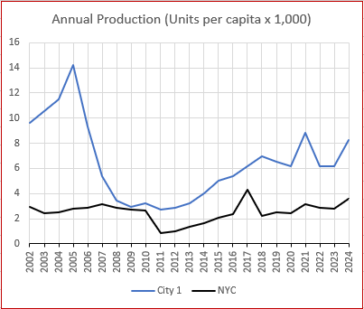
Figure 4 compares the lot premium for this city with the lot premium for New York City. I have also added a third city, to demonstrate the various paths cities have taken since 2000. Lots in New York City are perpetually inflated because supply constraints create elevated rents, and elevated rents justify paying a premium for land.

The mortgage crackdown reduced the marginal lot value in New York City just as it did in most cities, but since local supply constraints have pushed lot values so high in New York City, the marginal lot still had value well above zero.

Figure 4

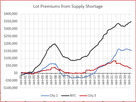
Figure 5 compares annual new home production in the sample city and in New York City. New York City’s rate of new home production is always very low, but since lot values remained above zero, the mortgage crackdown didn’t create a market breakdown there. After a brief decline, new home construction recovered back to the level of about 3 units per thousand residents. That’s where local willingness to approve supply maxes out in New York City.

This sample city does not limit supply so completely. So, how could it have possibly accumulated such a premium after 2015?

In the sample city, construction fell by more than 70%. If the mortgage crackdown hadn’t happened and if the Fed had aimed for recovery in 2008, housing production in the target city would have likely recovered quickly back up to 8 new units per thousand residents or more. In the 1970s, when construction activity was very cyclical, moves like that were common. When short-term cyclical fluctuations lead to reduced activity, capacity is available to reclaim quickly. By 2015, construction capacity had been permanently lost. Now, annual growth was limited by the difficult task of investing in new capacity.

Figure 5

From 2013 to 2018, new home production in the sample city increased steadily. By 2016, lot values were reliably positive. By 2016, lot values weren’t the constraint limiting new construction. Capacity growth was.

Estimating the Cumulative Supply Shortage

The next step in the model is using the lot premium to estimate the amount of construction required to keep rent inflation neutral. In the sample city, by the mid 2010s, demand from population growth and household formation had returned to levels similar to the 2000s. Construction rates were growing, but couldn’t grow quickly enough to meet the demand that returned as the economy returned to expansion. Then supply chain disruptions associated with Covid and with competition for resources from the AI boom and construction of manufacturing facilities further delayed growth of new home construction.

Figure 6 & the associated data are included in the package.

Figure 6

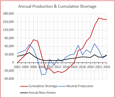
The number of new homes required to reverse post-2008 rent inflation and price inflation has grown to more than 150,000 units in the sample city, by my estimate. For the foreseeable future, the state of the housing market in the sample city will be a balancing act. How fast can construction capacity rise? How much of an effect will that have on rents, prices, and the unsustainable premium that lots in the sample city currently fetch? For developers and builders, this will be an odd time. There is near unquenchable demand for new homes, but in some markets those homes may lead to tight margins because land values will be declining as new neighborhoods are constructed. This data can identify markets where long-term acquisitions of land may be fruitful versus markets where work of significant quantity is available, but where getting in and out fast will be key.

These are key questions these analytical packages are meant to help you estimate.

How fast can construction capacity rise? How much of an effect will that have on rents, prices, and the unsustainable premium that lots in the sample city currently fetch?

This data can identify markets where long-term acquisitions may be fruitful versus markets where work of significant quantity is available, but where getting in and out fast will be key.

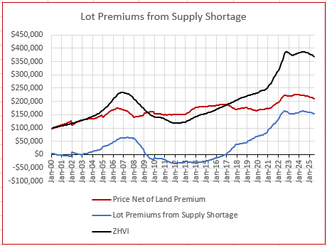
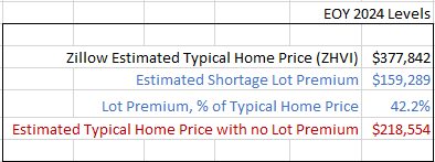
Figure 7 shows the price of the typical home in the sample city over time (the ZHVI, tracked by Zillow). It disaggregates that value between the lot premium (blue line) and traditional sources of value, like size, quality, and location (red line). Nearly half the price of the typical home in the sample city is now associated with the unsustainable premium.

Figure 7 & the associated data are included in the package.

Figure 7

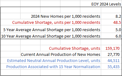
Every market has a different lot premium. Every city has a different neutral production level, associated with flattening rent inflation and flattening lot premiums. Every city has a different distance between current production and neutral production.

The lot premium is a relatively precise piece of information. It is based on the values of existing homes. One basic, and dependable, use for this number would be to combine it with local expertise in land markets. In this sample market, is that marginal land at the edge of town, prepped and ready for residential construction, selling for the equivalent of $159,000 per lot? Or is it selling at a discount to that? If it is, then the land might be developed profitably even if the land premium starts to decline while the project is being completed.

I suspect there are overlooked markets with positive lot premiums where there hasn’t been much recovery in new home construction, where the lot premium justified by home prices is, say, $40,000, but that premium isn’t reflected in land prices because there hasn’t been an active new construction market.

This is one way local underwriting expertise can leverage this information.

The estimate of units short is slightly less precise because it requires estimating demand elasticity to derive the number of missing units from the lot premium. (How much does 1% more housing lower rents?) But, precision isn’t as necessary on that question, and over time, we can adjust our estimates as we learn from the data.

The estimate of the neutral number of units needed annually is slightly less precise than that, because it requires estimating the neutral rate of construction necessary to keep rents moderate. Cyclical conditions are constantly changing that number from year to year. So, estimating each market’s neutral construction rate is much like the Fed trying to guess the neutral interest rate target. But, comparison across markets can help develop this perspective. City 3 in Figure 4 is actually ahead of the sample city in this process. It completed as many new units in 2024 as it had in 2005 - enough so that lot premiums are declining. That pattern will be coming to all cities with lot premiums. Lot premiums will be coming down in most markets.

Many builders will say they don’t use this sort of analysis. Real estate is about location and execution. And in all of history before 2008, they were correct. It is understandable that operators focus on those issues. The scatterplots in Figure 2 are a mess. Everything important about building in those markets was about why dots weren’t on the regression lines. They were all over the place. Knowing how to identify what made locations and projects different and what could create value was the whole deal.

The scatterplots in Figure 3 are screaming “This is a different kind of market.” The things that used to be too unimportant to analyze are now more important than the whole deal used to be, and many of your competitors are simply leaving that competitive advantage for you to use.

The market in the sample city in Figure 3 will someday look like 2002 again. Tracking how soon that will be and what will happen on the pathway there will be exceedingly important while we are on that pathway. And millions of homes will be constructed on that pathway. Understanding this framework will point to where those new homes will produce reasonable profit.

More on this in following posts.

Please share this if you know developers, investors, or others who might appreciate this insight and be interested in these packages when I make them available.