October 2024 Residential Construction

A decade ago, when I started researching housing, it seemed like every week I would find some new surprising detail about how empirically confused the conventional wisdom was on the financial crisis. It was a really fun time to just follow my nose deeper into the topic with each new surprising finding.

These days, it’s sort of a different kind of fun. Each month, it seems like data on housing has been purposefully designed to confuse. And, that mental model I have been building for a decade is the cheat code.

It’s like I have a picture and everyone else has an unassembled jigsaw puzzle. Over the years I’ve had decent luck making contrarian investments. But, I’ve never felt such command over such a complex set of facts.

“Thank you” to the few of you who are interested enough in this topic to follow me down these rabbit holes and to spend the extensive effort frequently required to figure out what the hell I’m trying to communicate. I hope you all feel like you’ve got a cheat code too.

Home values and home prices

This month, in addition to the monthly numbers on housing construction, the quarterly numbers on construction by intent and design were updated through the 3rd quarter. They include square footage, intent to sell or rent, etc.

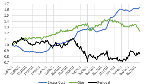
Here, I used average square footage and the BEA’s estimate of prices for residential investment in excess of the GDP price index.

The residual is basically the change in the prices of new homes that isn’t related proportionately to square footage or to input prices. It could be any number of things. Land costs, builder profits, changing quality of materials and upgrades, etc.

Since 1987, the average size of new homes has increased by 26% and the real cost per square foot has increased by about 37%.

Figure 1

The residual and the input price level are negatively correlated. That could be because of some measurement issue. Or it could be for some other reason. Maybe when prices of inputs rise, homebuyers react by reducing the quality and value of materials and upgrades.

In Figure 2, I chart the product of the residual and the excess cost. This is basically the real cost per square foot of new homes over time (black line). I also chart the real Case-Shiller index (red). The real increase in the cost of new homes per square foot is only about 1/3 of the increased cost of existing homes.

Furthermore, using Erdmann Housing Tracker data, I chart the real price of a ZIP code with no supply or credit access issues. This would generally be the richest ZIP codes in a city. This is a bit tricky because the variance of incomes across ZIP codes has increased substantially since the tracker data started in 2002. So, the solid blue line is a ZIP code with 90% percentile income. (Reported incomes in the 90th percentile ZIP code have grown much more than the average, since 2002.) The dotted blue line is a ZIP code with no supply or credit access sensitivity, with income growth since 2002 equal to average income growth.

The average ZIP code is the orange line. The difference in home price appreciation between the average ZIP code and the ZIP codes represented by blue lines is that the average ZIP code is affected by constrained supply (which inflates the price) and credit (which lowers the price).

The price trends based on tracker data begin in 2002.

Figure 2

I’m not quite sure how to interpret the high end housing measures (the blue lines) here. Over time, home values should be rising, but excess costs are due to a lack of productivity in construction. In a market with normal productivity growth and level real costs, the blue lines would still go up, and the difference between the black and blue lines would be larger homes. The relative trends in prices and the residual parts of home values suggests that rising construction costs are an important factor in the price of new homes in high-tier markets.

The average new home is smaller today than it was in 2005, even after the bottom half of the new home market was collapsed with the mortgage crackdown. That suggests, strongly, that high costs are changing the character of new homes. Home prices are pretty neutral as a multiple of incomes in the richest ZIP codes, but the size and quality of new homes in those ZIP codes has not kept up with rising real incomes.

Rising costs on the average home have very little to do with high construction costs. If they did, their home prices would be tracking new home prices. Average families are paying more for existing homes because their land value is inflated by the lack of supply.

Inadequate supply causes regressive rent and price inflation. Markets for rich homebuyers are tracking new home costs. Markets for average homebuyers are tracking existing home costs.

A rising cost of construction affects the characteristics of new homes in the high end market. A rising cost of land affects what average homes, whose characteristics are already set, sell for.

Details about this month’s new numbers are below.