Housing Supply, Costs, and Urban Value (Part 1)

Los Angeles, Seattle, and Austin

This will be an occasional series, possibly quite extensive by the time I am done, where I will explore how much of high housing costs are due to a lack of supply and how much are due to demand specific to a city. Some of this probably could be fodder for a more formal paper, but for now, it will be a series here at EHT.

I will probably eventually get into whether upzoning causes urban land values to increase or decrease. Piecemeal upzoning can cause specific land values to increase (like increasing the sales capacity on an alcohol retail license), but universal upzoning would cause land values to decline (like getting rid of alcohol retail licenses). The broader the upzoning, the more rare it would be for the land on any given property to increase in value. It is clear to me that broad upzoning (or otherwise removing barriers to new housing), would greatly reduce the aggregate land value in cities that are currently undersupplied. But, I hope to eventually lend some empirical backing to that intuition.

Austin, Los Angeles, and Seattle

Here, in part 1, I am just going to walk through a back of the envelope comparison of Los Angeles, Seattle, and Austin, to answer the question, “Is Los Angeles more expensive than Austin because there is more demand for living in Los Angeles, or because there isn’t enough housing?” In other words, if Los Angeles built as many homes as Austin, would it be as cheap as Austin? Is Los Angeles a superstar, or a stick in the mud?

I picked these three cities because they are all sometimes cited as “superstar” cities. There is no question that there is above average demand for residency in each of them. Can we come up with a ballpark estimate of how much demand there would be if housing supply was not artificially constrained?

Curvy Supply & Demand

I think these three cities basically lie at the three nodes of American housing. Austin has been taking in a lot of demand, but it is still basically a city that builds to grow, so rents remain relatively low, especially as a percent of resident incomes. Seattle builds moderately. Not enough to stay inexpensive, but enough to still grow. LA doesn’t build, and so, it is basically at the frontier of unaffordability. As it becomes more unaffordable, on the margin, residents don’t pay higher rents. They move away from the city entirely so that someone with a higher income can pay the higher rents.

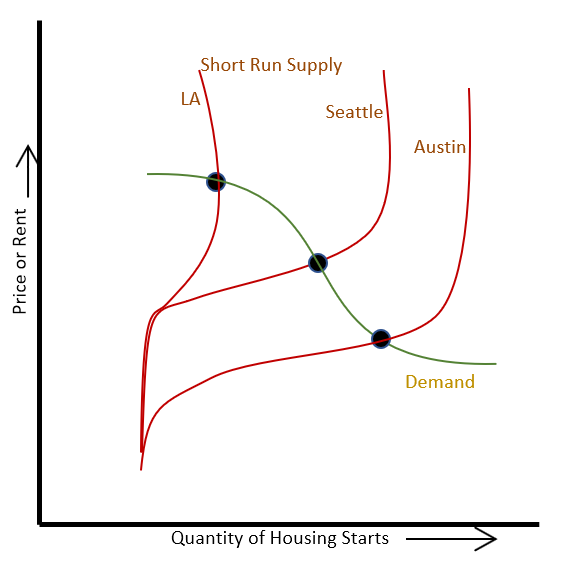
Basically, I think, metro area housing supply and demand curves are both non-linear in important ways, as shown in Figure 1. Supply is inelastic downward because the existing housing stock is permanent. Then, each metro area has a range where they are willing and capable of building more homes in a given period of time. Within that range, supply is elastic, with some marginal differences based on local permitting processes, etc. Then, each metro area has a maximum where they can’t approve more homes, and supply becomes inelastic again. Every city has been in that condition to an extent during the Covid period, but Austin was probably tickling that condition locally in any case also, because growth was very high.

As an aside, I think supply can actually start to turn backward and slope downward in the worst cases. (“You can’t build those houses. They’re too expensive!” on the left tip of the political horseshoe, and “We’ve worked hard to make this city nice. That’s why people are willing to pay more to live here. Now, you’re going to dilute that?” on the right tip of the political horseshoe.)

Figure 1 - demand from existing residents

So, Austin, Seattle, and Los Angeles all might exist on the same basic demand curve. In Austin, the supply curve crosses it where demand is elastic. If Austin built more, household spending for housing, for both rich and poor, would tend to reflect comfortable choice. Typically, in those conditions, home prices settle around 3-4x incomes.

In Seattle, the supply curve crosses demand where demand is inelastic. Residents are willing to spend more to stay. They don’t want to. But they can. So, if Seattle built more, the typical resident would spend less. If Seattle built more homes, rents would decline.

In LA, the supply curve crosses demand where demand is elastic again. Here, elastic demand means that the family on the margin leaves the city entirely. Demand is expressed through migration rather than marginal choices on spending. If LA built more homes, it might not have that much of an effect on rents at first. Initially, there would be a boost in demand because families who would have been displaced might decide to stay, even if rents just stabilized.

The Price/Income Slope

In “Price Is the Medium Through Which Housing Filters Up and Down: A Proposal for Price/Income as an Indicator of Housing Supply Elasticity”, I discussed the tendency of inadequate supply to create a pattern in home prices that is highly sensitive to incomes.

You can infer this pattern from Figure 1. Figure 1 is an aggregate demand curve, but within each city, that curve is made up of families at various points on the curve. Spending on housing is very dependent on income. So, where costs are rising, poor families start moving to the top left of the demand curve before rich families do.

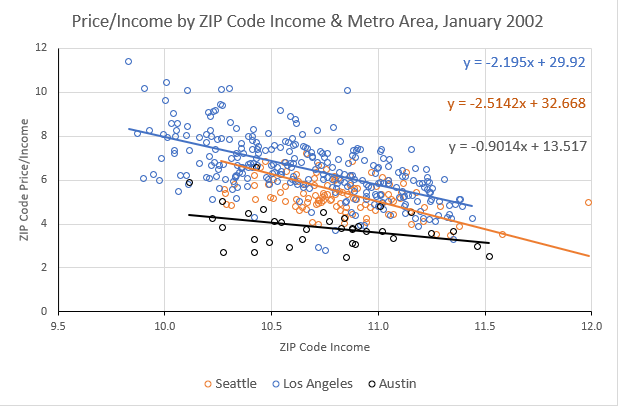
In 2002, shown in Figure 2, every family in Austin (speaking broadly) was basically at the right end of Figure 1, in the happy comfortable range.

In Seattle and Los Angeles, families have to climb up that demand curve to higher rents as they get outbid by families with higher incomes who can spend more on the available housing. Every family has a different breaking point, where their demand for living in a location - for not being displaced - turns their local demand curve flat. In each ZIP code, working right to left, the demand curve will generally be inelastic (more vertical in figure 1) and you will find an increasing number of families making that choice - either trading down into the lower-tier local neighborhoods or moving out of the metro entirely.

Figure 2 (incomes are ZIP code average, on natural log scale, 10=$22,000, 11=$60,000)

Figure 3 shows the state of housing affordability in these three cities today. They have all gotten worse. (We stopped the big bad housing boom, don’t ya know?) And, here, you can see LA in the condition described in Figure 1. I suspect that price/income ratios above the mid-teens is just not a range any city is going to exceed. There is a limit to how much families can spend and to how quickly they can move into and out of a region. At this point, families in those dots on the top are pretty hastily (on a macroeconomic scale) getting to the business of moving to Arizona or Texas. The hardest job in the country right now is the executive in charge of getting U-Haul trucks back to LA.

Figure 3 (incomes are ZIP code avg, on natural log scale, 11=$60,000, 12=$162,000)

In the paper, in regressions between migration and the price/income slope shown in Figures 2 and 3, each 1 point decline in the slope was associated with an annual outmigration of 0.38% of the population. There was no significant relationship between the slope and rates of inmigration.

In other words, again broadly speaking, incoming residents have elastic demand. They have a reason for coming, and they aren’t as deterred by the cost. When they come, you can either build a house or empty an existing house for them. The way an existing house is emptied is that costs rise, as they interact with those non-linear demand curves, until some family hits that flat part at the top left of Figure 1, moves away, and a home is now empty.

So, as I discussed in the paper, home values aren’t really determined by a standard static financial formula anymore. They are determined by flows. How expensive does it need to get in order for x number of families to choose displacement. And, I quantified the process by which that happens. Home prices have to rise 1 point per log point of income (the difference in the price/income between say 12 and 11 on the figures), to get 0.38% of the population to leave.

Superstar or Second-Rate?

Maybe this model can help estimate the high cost that is due to high demand vs. low supply.

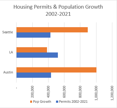
Figure 4 compares permits issued and population growth from 2002 to 2021 in these metro areas. In absolute numbers, they have all approved about the same number of permits over those 20 years, but Seattle and Austin have added a lot more people.

Figure 4

This creates some confusion. Some people see this as evidence that there isn’t a housing shortage. LA built more than one house for each additional resident over 20 years. So, some will mistakenly say high prices are due to low interest rates, local amenities, speculation, etc.

At the other end of the spectrum, you’ll hear that LA is expensive because it’s just so fantastic. So many people just want to live there. It’s a “superstar”.

Of course, the rate of new building is very low in LA. It’s a much larger city than the other two.

Both of these those theories can’t be true. It can’t be that LA is building more than enough at such low levels, and it is expensive because there is just too much demand to keep up with.

In fact, both claims are wrong.

If you assume that the existing stock of homes lost about 7% of its capacity over the last 20 years (through changing household size, the loss or replacement of old homes, etc.) so that a small amount of building is required just to keep population level, then after accounting for that small loss rate, all three cities have grown by about 2.5 residents per new home. That happens to be roughly the US average household size.

In cities like LA that are stagnant, changes in the condition and use of the existing stock of homes become more important factors determining population growth than new building is. LA built so few new homes that most of them were just replacing lost home or were providing shelter for a stagnant population.

Let’s think of housing supply required to meet demand for living in a city as being composed of 2 parts. (1) Build a new home (2) empty an existing home. Add up those two parts, and that is the potential population growth that the city had to match in order to create a home for all of families who wanted to live there. In other words, that is the number of homes that needed to be available to meet demand - either built new without creating regional displacement or carved out of the existing stock as a result of displacement.

This is a rough approximation, but in Figure 5 I estimated the unmet potential by multiplying the average price/income slope* x 0.38 x 20 years for each city. That, plus the actual number of homes built, equals the estimated demand that the city was faced with.

So, the blue bar is the population growth rate over twenty years, which reflects the number of homes built. The middle light gray bar is the estimated population growth that would have accompanied ample home building. The bottom bar is an alternative measure that accounts for the effect of property taxes on home values and the price/income slope.

This probably understates demand for living in LA. In my paper, the estimate of the correlation between new homes and inmigration was not statistically significant, but it also wasn’t necessarily zero. A lack of homes must slow down inmigration somewhat, though. That’s a difficult quantity to estimate.

I would say that the incomers must have less elastic demand (are less price-sensitive) than the leavers. But that is only based on the decisions of the actual incomers. Of course the potential incomers who were more price sensitive didn’t come. How many of them are there? How would you count them?

The lack of a strong correlation between a steeper price/income slope and the inmigration rate (from the paper) suggests that the potential additional population growth from blocked incomers is positive, but less than the number of leavers. In other words, the gray bars account for most of the potential demand that was limited by housing supply.

And, so that leaves us with an estimate that of these three cities, Austin is the most “super”. If housing was amply supplied, Austin would have grown more than Seattle and LA over the last twenty years, and it did grow at a rate pretty close to that potential.

Whereas Austin’s potential was something like 80%, Seattle was probably closer to 55% (broadly accounting for repelled potential incomes), and LA was likely around 45%. US growth was about 16% over those 20 years, so the demand for living in all three of these cities is above average.

On the building side, Austin is well above average, Seattle somewhat above average, and Los Angeles is about as far below average as you can get. LA might need to act like an above average city to become affordable, but the bar isn’t that high. Most of their problem is from a severe lack of building.

* I used a slope of -0.7 as the neutral benchmark. Supply induced outmigration was inferred from any slope steeper than that.